OECD global long-run economic scenarios: 2025 update

时间：2025-09-04

Abstract

This paper describes the latest update of the OECD’s long-term scenarios, which are done every 2-3 years to quantify some of the most important long-term macroeconomic trends and policy challenges facing the global economy. The focus is on illustrating the output trade-off associated with transitioning to low-carbon energy sources, between the shorter-run costs of carbon mitigation and the longer-run benefits of avoided climate damages. Both are subject to considerable uncertainty, which is illustrated using several scenarios that vary according to the steepness of the climate damage curve and how quickly carbon mitigation costs decline. The paper includes two annexes detailing the changes that have been made to the projection framework, the first on the expanded country coverage and revised productivity convergence framework and the second on the new climate damage channel.

Acknowledgements

This paper has been prepared by Yvan Guillemette.

An earlier version of this policy paper was discussed at a meeting of Working Party No.1 (WP1) of the OECD Economic Policy Committee. The meeting participants, as well as Diogo Baptista, Sebastian Barnes, Jean Château, Hélia Costa, Alain de Serres, Åsa Johansson, Tobias Kruse, Nigel Pain, Pierre-Alain Pionnier, Mauro Pisu, Sébastien Turban, David Turner, D. Filiz Unsal and Volker Ziemann provided comments on earlier versions of the paper. Thomas Chalaux helped with demographic projections, Isabelle Fakih and Veronica Humi with editorial assistance, Patrice Orliange and Casper Meyer Zu Schlochtern with database assistance and Steven Cassimon and Wendy Stokle with release materials and data visualisations.

Main findings

This paper presents updated and extended long-run economic scenarios. The projection horizon has been extended to 2100 and the underlying Long-Term Model now incorporates the full global economy, a revised supply-side framework, and allows for the impact of climate damages on output. To highlight some of the uncertainties about the costs and benefits of the climate transition, the paper considers six scenarios with differing assumptions about the speed of the energy transition, the pace at which carbon mitigation costs decline and the extent of climate damages.

Energy transition scenarios

In the energy transition scenarios, all countries accelerate decarbonisation and energy efficiency efforts, eliminating coal as an energy source by 2050 and lowering the shares of oil and gas in primary energy to 5% and 10%, respectively, by then. This scenario limits the global temperature increase to 1.6°C by 2100, meeting the Paris climate agreement goal.

The impact of the global energy transition on output trajectories is highly uncertain. Four scenarios illustrate different possibilities:

With a median climate damage curve and a slow decline in mitigation costs, global output remains lower in 2100 than in the corresponding business-as-usual scenario.

With a median climate damage curve and a quick decline in mitigation costs, the energy transition becomes a net positive for global output around 2085.

With a high-damage curve and a slow decline in mitigation costs, the energy transition becomes a net positive for global output in the mid-2050s.

With a high-damage curve and a quick decline in mitigation costs, the energy transition becomes a net positive for global output in the mid-2040s. All 139 countries modelled individually are net beneficiaries by 2080.

In terms of projected levels of global potential output per capita, the scenario with a median climate damage curve and a quick decline in mitigation costs presents the most optimistic outlook, with global living standards higher than in the business-as-usual counterpart by the end of the century.

1. Introduction

1. Long-run economic projections are essential to address evolving long-term challenges with well-designed policies. Such challenges can be global, as with climate change, national, with governments needing to ensure that social security, healthcare, and education systems remain sustainable over the long term, or regional, with the need to design infrastructure and urban development plans that can accommodate future population growth and economic changes. Actuaries and financial planners also need to consider long-run economic trends to advise on investment and pension plan choices.

2. To help make informed decisions in these fields and many others, the OECD publishes long-run scenarios every two to three years that illustrate some of the most important economic trends and policy challenges facing the global economy and how they might evolve over time.1 Relative to other sources of long-run projections, the main value added of the OECD ones is to provide results at the country level for a large number of economies using a common, relatively simple and tractable framework. Frequent updates also ensure that the scenarios incorporate and start from up-to-date historical data and estimates.

3. One of the central long-run challenges facing the global economy today is the need to accelerate the transition toward renewable energy sources to reduce greenhouse gas (GHG) emissions and attenuate the impacts of climate change. An illustration of the potential impacts of an accelerated transition on future output trajectories must consider two main impact channels. The first is faster carbon mitigation, a negative supply shock in the short to medium run. The second is the avoidance of climate-related damages, a positive supply shock in the medium to long run. However, projections of these channels are unavoidably sensitive to a range of conditioning assumptions that are hard to distinguish on historical data. This enormous uncertainty presents a challenge for scenario building. To highlight some of the uncertainties surrounding both costs and benefits of the energy transition, this paper considers six scenarios with differing assumptions about the speed of the transition, the pace at which carbon mitigation costs decline and the extent of climate damages (Figure 1).

4. The paper is organised in three parts:

Section 2 presents a baseline business-as-usual scenario (BAU1 in Figure 1) in which the energy transition continues at its recent historical pace, which is not sufficient to limit the global temperature increase to well below 2°C as ambitioned in the Paris climate agreement. For the first time, the reduction in output associated with projected climate damages is illustrated, initially using a median climate damage curve. Carbon mitigation costs are absent by design. This scenario is presented in some detail to illustrate the full set of changes that have been made to the projection framework in the Long-Term Model (LTM) and because, except for the addition of a climate-damage channel, it is the one most directly comparable to previous baseline scenarios (Guillemette and Château, 2023[1]). The sensitivity of potential output projections to the choice of a climate damage curve is then illustrated using an alternative business-as-usual scenario with a steeper climate damage curve (BAU2 in Figure 1).
Section 3 outlines alternative scenarios in which the global community successfully transitions to low-carbon energy by 2050 and keeps the global temperature increase to below 2°C. Faster carbon mitigation weighs on output – according to the carbon abatement cost curves introduced in the previous vintage of the LTM – but also provides economic benefits by attenuating global warming. The net effect depends on both how fast carbon mitigation costs are assumed to decline over time and how much climate damages are avoided. Four energy transition scenarios are considered that make different assumptions along these two dimensions. The net benefit of the transition and its dynamics are illustrated by contrasting the global output trajectory in the four energy transition scenarios (ET1 to ET4) with that of the BAU scenario that relies on the same damage curve assumption (as illustrated by the connecting lines in Figure 1).

5. Box 1 provides an overview of the core part of the LTM and Annexes B and C detail the new changes made to the model and their underpinnings. Many of these extensions and updates are interrelated. Notably,

The geographical coverage of the LTM has been extended to be able to produce and analyse global scenarios. In addition to the 49 countries that were already present in the model, 90 have been added individually using a simplified approach and 55 have been added as part of three regions. These new countries and regions are typically not shown individually, however, but they are used to decompose global outturns to the regional level following World Bank regional groupings. Annex A summarises the classification of countries into regional groupings.
The geographical coverage of the LTM has been extended to be able to produce and analyse global scenarios. In addition to the 49 countries that were already present in the model, 90 have been added individually using a simplified approach and 55 have been added as part of three regions. These new countries and regions are typically not shown individually, however, but they are used to decompose global outturns to the regional level following World Bank regional groupings. Annex A summarises the classification of countries into regional groupings.
The projection framework has changed. The inclusion of a broader range of countries at different stages of development, the resulting data gaps, and the desire to preserve a common approach across countries has necessitated new analytical work and revisions to the previous framework. Most notably, the convergence mechanism for trend labour efficiency has been revised. In addition, the definition of the capital stock has changed to include dwellings, which alters both the starting point for the level of the capital stock and that for trend labour efficiency, since the latter is calculated as a residual.
The projection horizon has been extended from 2060 to 2100, which helps to illustrate differences in global warming across scenarios given the slow dynamics of the carbon cycle. This extension also allows OECD scenarios to be used as inputs into other analyses with a long projection horizon.
The output costs associated with climate damages are considered for the first time.

Box 1. The framework for potential output projections and decompositions

The OECD Long-Term Modem (LTM) consists of a set of dynamic projection rules and identities for variables of interest, implemented at the country level using annual data. For all countries, the backbone of the model is potential output, assumed to be a function of available inputs (labour and capital) and the efficiency with which those inputs are combined (labour efficiency). The production function is a constant-returns-to-scale Cobb-Douglas function with Harrod-neutral labour-augmenting technical progress. Indexing country and time with subscripts [Math Processing Error] and [Math Processing Error] (annual frequency) and using mnemonics as they appear in OECD Economic Outlook (EO) databases, potential output ([Math Processing Error]) is:

[Math Processing Error]

where [Math Processing Error] denotes trend employment; [Math Processing Error] represents a whole-economy measure of the capital stock, [Math Processing Error] is trend labour efficiency and [Math Processing Error] is the labour income share, assumed to be 0.67 in all countries. For the countries covered directly in the EO, potential output projections are an extension of the short-term potential output estimates prepared for the EO. A similar but simplified approach, described in Annex B, is used to estimate and project potential output for other countries using historical data from the World Bank’s World Development Indicators (WDI) database. The last historical period in these different sources is the starting point for long-run projections and is referred to as the jump-off point (between historical and projection periods). Potential output is projected out to 2100 by modelling the trend input components separately.

Trend labour efficiency

Trend labour efficiency is projected using a revised framework that mixes elements of absolute and conditional convergence. Convergence is absolute in so far as trend labour efficiency in every economy is ultimately going to a common frontier level. And it is conditional in so far as the speed at which this occurs is a function of country-specific framework conditions. The revised framework is based on a model estimated over the 1996-to-2023 period using data for the 139 individual countries included in the LTM. The model and estimation results are detailed in section B4 of Annex B. The estimated coefficients are then incorporated in the closely related projection equation:

[Math Processing Error]

where [Math Processing Error] is log trend labour efficiency expressed in USD at fixed 2021 prices and Purchasing Power Parity exchange rates ([Math Processing Error]). Its projected growth rate ([Math Processing Error]) is the sum of five components:

Rate of global technical progress (). This component is common to all countries and set to 1% in the scenarios examined in this paper. This assumption is based on the geometric mean trend labour efficiency growth rate of advanced G20 economies over the past 30 years or so.

Rate of global technical progress ([Math Processing Error]). This component is common to all countries and set to 1% in the scenarios examined in this paper. This assumption is based on the geometric mean trend labour efficiency growth rate of advanced G20 economies over the past 30 years or so.
Convergence to frontier ([Math Processing Error]). This component captures the effect of catching up toward the frontier labour efficiency level ([Math Processing Error]), assumed to be that of the United States, or a country’s own level if already higher than that of the United States. In the latter case the convergence term is zero by construction (this applies to only a handful of economies, notably oil-rich ones). The growth impetus depends on how far a country is relative to the frontier [Math Processing Error] and on a country-specific speed of convergence ([Math Processing Error]), which is modelled as a function of a country’s framework conditions. Those include the quality of governance (based on the World Bank’s Rule of Law indicator, [Math Processing Error]), the degree of economic globalisation (based on the KOF Swiss Institute’s economic globalisation index, [Math Processing Error]) and an index of macroeconomic stability (based on the level and variance of a moving average of headline inflation, [Math Processing Error]). The need for tractability, broad country coverage and avoidance of data gaps has led to the selection of only three framework conditions but, in practice, these proxy a wider set of correlated structural growth determinants. A country with mean scores on all three structural indicators would close approximately 1.3% of any remaining gap with frontier labour efficiency annually. Better scores on the structural indicators raise this speed and vice-versa (based on estimated coefficients [Math Processing Error], [Math Processing Error] and [Math Processing Error]). Implied convergence speeds at the jump-off point vary between zero (no convergence) to 2.6% annually. Framework conditions are assumed to remain at initial values in the scenarios examined in this paper, as has been the convention in previous exercises, so convergence speeds do as well.
Climate damage ([Math Processing Error]). The output costs associated with global warming are assumed to manifest primarily via lower trend labour efficiency (with knock-on effects on capital accumulation). See Annex C for additional details.
Carbon abatement costs ([Math Processing Error]). In the BAU scenarios, abatement costs are set to zero by design. In energy transition scenarios, abatement of carbon emissions is assumed to impact trend labour efficiency according to country-specific elasticities of output to carbon mitigation. These elasticities are estimated from a range of scenarios produced with the ENV-Linkages model (Château, Dellink and Lanzi, 2014[2]). These elasticities reflect the state of technology today, so a parameter can be adjusted that controls the rate at which carbon abatement costs are assumed to decline over time. See Annex B of Guillemette and Château (2023[1]) for additional details.
Momentum ([Math Processing Error]). This residual component captures that part of trend labour efficiency growth at the jump-off point that is unexplained by other components of the model. The initial value decays over time with a half-life of about 6 years (based on estimated coefficient [Math Processing Error]). This decay rate ensures a smooth transition from estimated trend labour efficiency growth rates at the jump-off point and longer-run projections. Given the parsimoniousness of the specification, the momentum component captures many country-specific growth determinants beyond those affecting the speed of convergence. The gradual decline of this component implicitly assumes that these determinants are persistent, but not permanent.

In the very long run, save for the impact of mitigation or climate damages, trend labour efficiency growth in all countries converges to the assumed exogenous rate of global technological progress (1% per annum), although for most countries this would occur beyond the 2100 projection horizon.

Trend employment

The evolution of trend employment is primarily the result of three sets of dynamics: the evolving size of the working-age population (defined here as ages 15 to 74); its age composition; and trends in the employment rates of different age/sex groups. The size and composition of the working age population follows the demographic projections of the United Nations World Population Prospects (2024 revision, medium variant) and are exogenous in the LTM. Trends in the employment rates of different age/sex groups are projected by applying a cohort approach to historical employment rates (Cavalleri and Guillemette, 2017[3]). These generational trends reflect societal changes, such as rising female employment rates, but also structural changes such as higher educational attainment. Already-legislated future changes in legal retirement ages are incorporated in projections of the employment rates of people aged 55 and over. Climate damages are assumed not to affect population size or potential employment, although heat-related mortality and international migration could be important drivers of climate-related output costs in some countries.

Capital stock

In the short to medium run, the main source of variation in the capital stock is the net investment rate at the jump-off point. If it is higher than the rate that would be consistent with keeping the initial capital-to-output ratio stable given projections of trend employment and trend labour efficiency growth, then the capital-to-output ratio rises and contributes positively to potential output growth, and vice-versa. In the longer run, investment rates adjust dynamically to target a capital-to-output ratio of 3.4, an historical average among advanced countries. This adjustment happens very gradually, and the target is not attained by all countries by the end of the projection period. The fixed long-run target for the capital-to-output ratio implies that both climate damages and carbon abatement impact the level of the capital stock proportionally. In equilibrium, given the 0.33 capital income share in the production function, one third of climate damages and one third of any carbon abatement costs come through via a lower ratio of capital per worker.

Potential output per capita growth decomposition

A convenient expository decomposition (used in figures) is to divide changes in potential output per capita, a crude metric for living standards, into productivity, capital intensity and labour utilisation components:

[Math Processing Error]

where [Math Processing Error] is log potential output per capita, [Math Processing Error] is log trend working-age population, [Math Processing Error] is log trend total population and other lower-case variables are logarithms of their upper-case counterparts introduced above. The first term on the right-hand side of this equation measures the contribution of trend labour efficiency growth to potential GDP per capita growth; the second term measures the contribution of capital intensity (capital per worker); the third picks up the contribution of the trend employment rate; and the last term indicates the contribution of the working-age population share, a summary indicator of the population age structure.

6. Long-run scenarios should not be treated as predictions of the future but rather as illustrations of some of the long-run challenges facing the global economy, how they might evolve, and how they might affect different countries. Differences in projections relative to earlier vintages should not be interpreted as the result of policy action, or inaction, in the interim period, nor as necessarily indicating a reassessment of a country’s growth prospects as they are more likely to stem from new national accounts data, and changes in methodology and assumptions. Moreover, The LTM relies on many different sources of data and in some of these sources the last available data points are for 2022 or 2023. Therefore, recent policy changes are not always reflected fully in the analysis, and this includes recent changes to trade policies and tariff rates. Annex A goes over other important caveats inherent in the use of such a stylised tool.

2. Baseline business-as-usual scenario (BAU1): slower global potential growth in a warming world

7. The BAU1 scenario generally assumes no change to initial policy and institutional settings, except where already-legislated reforms will have a known impact on the policy indicators included in the framework, such as future changes to statutory retirement ages. In addition, every country is assumed to undertake, as of 2027, a gradual fiscal adjustment sufficient to eventually stabilise government debt as a share of GDP at its projected 2026 level.

2.1. Global output growth continues to moderate and greenhouse gas emissions only fall slowly

8. From around 2.9% currently, global annual potential output growth is projected to moderate gradually, to 2.7% in the first part of the 2030s, 2.1% in the early 2040s and around 1.3% in the latter part of the century (Figure 2, Panel A). Much of this trend is attributable to demographic factors (see below). All regions other than sub-Saharan Africa contribute to this slowdown, but East Asia and Pacific disproportionately so: its growth contribution declines from more than one percentage point (pp) today to less than a fifth of a percentage point by the end of the century. China accounts for most of this slowdown, its individual contribution to global annual growth falling from about 0.9 pp today – almost a third of global growth – to zero by the late 2050s. This development does not happen uniformly over time – the share of East Asia and Pacific in global output continues to rise through to the early-2030s before starting to decline gradually. The two regions gaining in global output shares over the long run are South Asia (driven largely by India) and sub-Saharan Africa, the latter projected to account for some 13% of global output by the end of the projection period compared to 3% today (Figure 2, Panel B). Measured in US dollars at fixed 2021 Purchasing Power Parity (PPP) exchange rates, China has been the largest economy in the world since 2016 and is projected to remain so until the mid-2060s when it is surpassed by India.

Note: In Panels A and B, aggregates are computed using fixed 2021 Purchasing Power Parity exchange rates. In Panel C, historical data on energy mix are from the IEA’s World Energy Balances database. In Panel D, CO2 emissions from energy use and industrial processes and are projected on the basis of output and the energy mix. Other GHG emissions include all other sources (except land use change and forestry) and are projected at the country level on the basis of population, living standards and a time trend. See Annex A and references therein for methodological details.

Source: OECD Economic Outlook 117 long-term scenarios database.

9. In the BAU1 scenario, decarbonisation of the global energy mix continues at the recent historical pace, an assumption implemented by making country-level primary energy mixes continue to evolve along time trends estimated over the past two decades. This implies energy substitution that is clearly insufficient to reach a global net zero GHG emissions objective in this century as carbon-based sources still account for three quarters of the global primary energy mix in 2050 and more than 60% in 2100 (Figure 2, Panel C). Given the slowly changing energy mix, and despite an assumption of continued improvement in energy efficiency, global net GHG emissions are projected to keep increasing through around 2040 before starting to decline (Figure 2, Panel D).2 Peak oil occurs in the mid-2040s.3 Negative emissions, such as carbon capture and storage, are assumed to have only a small impact on global GHG emissions up to 2050 but reduce net emissions to a greater degree thereafter.

10. Insufficiently rapid progress on reducing GHG emissions implies continued global warming. The LTM now includes a simplified global carbon cycle, according to which the global surface average temperature anomaly (compared to the pre-industrial era) continues to increase throughout the projection period and reaches 2½ °C in 2100 (Figure 2, Panel E). As a result, the global output loss associated with climate change, estimated at approximately 1¾ per cent of global GDP today, rises to nearly 9% by 2100 (Figure 2, Panel F). The global climate damage projection is perhaps the most uncertain aspect of this exercise. The BAU1 scenario is based on a stylised median damage curve within the wide range proposed in the scientific literature. Section 2.6 below summarises the modelling approach and illustrates the sizeable impact on future output projections of using a steeper climate damage curve at the high end of that range (BAU2 scenario).

11. The climate damage channel in the LTM is intended to add greater realism to future output projections but not to evaluate the optimal speed at which GHG emissions should be reduced, or to provide definitive climate damage estimates for any one country. The chosen damage curve implies a social cost of carbon (SCC) of USD 253 at PPP exchange rates, within the range of many recent estimates, although some studies have estimated the SCC to be over USD 1 000 (Moore et al., 2024[4]). Moreover, the smoothness of the curve ignores potential tipping points in the global climate system that portend catastrophic climate and economic impacts. Avoiding such risks provides a central justification for accelerating efforts to reduce GHG emissions. Even if central estimates of future damages were not very high, it would remain desirable to reduce carbon emissions quickly based on risk arguments alone. Sections 2.6 and 3 partly illustrate these risks by considering scenarios with a much steeper global climate damage curve than the one used in the BAU1 scenario.

2.2. Global output per capita growth also slows but less than headline growth

12. Most of the projected slowdown in global potential output growth is attributable to slowing working-age population growth (working ages being defined as 15 to 74). According to the latest United Nations World Population Prospects (2024 revision, medium variant) on which all scenarios in this paper are built, the growth contribution of the trend working-age population component, currently around 1.2 pp, declines steadily and turns negative in the early-2080s (Figure 3, Panel A).

Note: Aggregates are computed using fixed 2021 Purchasing Power Parity exchange rates.

Source: OECD Economic Outlook 117 long-term scenarios database.

13. When looking at an output per capita measure, a concept more closely related to living standards, it is the projected decline in the working-age population share (of total population) that matters, and its growth contribution is essentially zero at the global level over the projection period (Figure 3, Panel B). As a result, the per capita measure slows by less than the headline measure, falling from about 2% annually today to 1¼ per cent by 2050 and remaining broadly stable thereafter. The rest of the BAU1 scenario presentation focuses on the period to 2050.

14. In the OECD area, annual growth in potential output per capita is projected to average 1½ per cent to 2050, but with substantial variation across countries (Figure 4, Panel A).

Projected average annual growth rates exceed 2% in a few countries (Chile, Costa Rica, Estonia, Greece, Lithuania, Latvia and Türkiye). Conversely, average annual growth rates are below 1% in only two countries (Luxembourg and Switzerland). These exceptions are mostly attributable to the trend labour efficiency growth component, which tends to be higher in countries that are more distant from the frontier level and which therefore have more scope to catch up over time, while those closer to or at the frontier level show a smaller contribution. This growth component is explained and decomposed further below.
In a few countries the pure demographic component (trend working-age population share) contributes positively to growth (e.g. Israel and Mexico), while in others it subtracts modestly, and as much as 0.7 pp annually in Korea.
Differences in the trend employment component across countries are due primarily to female employment dynamics and secondly to changes in the age structure of the working-age population, because employment rates tend to be lower in older age groups. The growth contribution of trend employment thus tends to be high where female employment rates have been rising steadily, as this trend is carried forward by the cohort model underpinning the projections (e.g. Korea) while it is close to zero where female employment rates are already high (e.g. Norway).
Differences in the capital stock per worker component are mainly due to differences in estimated capital-to-output ratios at the start of the projection period. Given that the underlying model targets a common capital-to-output ratio in the long run, countries with initially lower ratios tend to have more positive contributions from this component (e.g. Poland).

15. Growth in per capita potential output is substantially stronger in the G20 emerging economies than in the advanced economies, at 2.6 per cent on average annually between 2025 and 2050. This is driven in large part by China, India and Indonesia, despite a modestly negative demographic component in China (Figure 4, Panel B). The outsized growth contribution from the trend employment component in India (0.7 pp) is attributable to official data showing rising employment rates among women in recent years, and the remaining scope for further increases.4 India’s leading performance among the major economies also explains the relative outperformance of the South Asia region (Figure 4, Panel C). Sub-Saharan Africa is notable for being the only region with a substantially positive growth contribution from the working-age population share (0.5 pp).

Note: Aggregates are computed using fixed 2021 Purchasing Power Parity exchange rates. EA17 (Euro area) includes the 17 Euro area countries that are OECD members. G20ADV (G20 advanced) includes Australia, Canada, Germany, France, the United Kingdom, Italy, Japan, Korea and the United States. G20EME (G20 emerging) includes Argentina, Brazil, China, India, Indonesia, Mexico, Russia, Saudi Arabia, Türkiye and South Africa. Other acronyms are EAP (East Asia and Pacific), ECA (Europe and Central Asia), LAC (Latin America and Caribbean), MNE (Middle East and North Africa), NAR (North America), SAR (South Asia), SSA (Sub-Saharan Africa) and WLD (World). See Table A A.1 in Annex A for the composition of regional aggregates.

Source: OECD Economic Outlook 117 long-term scenarios database.

16. Relative to the last baseline scenario published in December 2023, changes to potential output per capita growth to 2050 are generally small in OECD countries (Figure 5, Panel A). Revisions to the trend employment rate component can usually be attributed to recent dynamics in employment rates (over the past 5 years or so). When those have been stronger than they had been when the previous vintage was done, the cohort-based approach tends to carry that strength forward in time, as in the United States and Greece. For other output components, the revisions are more difficult to decompose as, in addition to new data, they also reflect methodological changes made to the LTM.5 For this reason, they should not necessarily be interpreted as changes to a country’s growth prospects or a reflection of recent policy developments. For instance, Colombia and Mexico show sizeable downward revisions to annual average trend labour efficiency growth (see section 2.3 for a decomposition of the revision to this specific component).

Note: Aggregates are computed using fixed 2021 Purchasing Power Parity exchange rates. EA17 (Euro area) includes the 17 Euro area countries that are OECD members. See Table A A.1 in Annex A for the composition of regional aggregates.

Source: OECD Economic Outlook 114 and 117 long-term scenarios databases.

17. In selected non-OECD countries, revisions to potential output per capita growth to 2050 are larger than in OECD countries and generally driven by downward revisions to trend labour efficiency growth (Figure 5, Panel B). These are mostly associated with methodological changes and are decomposed and explained further in the next subsection. They are only partly compensated by upward revisions to trend employment rate projections, the most notable being that of India.

2.3. Labour efficiency is the main driver of future gains in output per capita

18. Trend labour efficiency is particularly important for growth within countries and is a key factor accounting for differences in potential output growth between countries. The projection framework for this growth component has been revised, in particular the drivers of cross-country convergence have changed. In addition, the projection framework now incorporates climate damages associated with the projected global temperature anomaly. The allocation of global damages to individual countries/regions is based on their relative vulnerability to global warming, which is a function of their specific climate and level of development (see section 2.6). It should be stressed nonetheless that this modelling is highly stylised and subject to evolve over time. Ongoing OECD analytical work will help to refine the individual-country estimates that are presented here to illustrate the revised framework.

19. At the global level, annual trend labour efficiency growth is projected to average 1.3% to 2050 (Figure 6, Panel C). Global technical progress, which is assumed to rise by 1% per annum, accounts for most of this result. The rest can be decomposed into three factors (see Box 1): a positive convergence component (0.6 pp annual average) owing to most countries being below the conceptual frontier level of labour efficiency and assumed to converge toward it over the period; a negative climate damage component (-0.1 pp annual average); and a negative momentum component (-0.2 pp annual average).

Note: See Box 1 for an explanation of the components in the legend. Aggregates are computed using fixed 2021 Purchasing Power Parity exchange rates. EA17 (Euro area) includes the 17 Euro area countries that are OECD members. G20ADV (G20 advanced) includes Australia, Canada, Germany, France, the United Kingdom, Italy, Japan, Korea and the United States. G20EME (G20 emerging) includes Argentina, Brazil, China, India, Indonesia, Mexico, Russia, Saudi Arabia, Türkiye and South Africa. Other acronyms are EAP (East Asia and Pacific), ECA (Europe and Central Asia), LAC (Latin America and Caribbean), MNE (Middle East and North Africa), NAR (North America), SAR (South Asia), SSA (Sub-Saharan Africa) and WLD (World). See Table A A.1 in Annex A for the composition of regional aggregates.

Source: OECD Economic Outlook 117 long-term scenarios database.

20. In the OECD area, average annual trend labour efficiency growth to 2050 is equal to the global outcome (1.3%) but one notable result is that many more OECD countries have negative momentum components than positive ones, and sometimes large ones (Figure 6, Panel A). This is because estimated trend labour efficiency growth rates at the jump-off point (between the historical and projection periods, currently 2026) are often lower than the convergence equation would predict. The prevalence of negative momentum is unsurprising in the context of the general slowdown in productivity growth observed across advanced economies in recent years, which a stylised catch-up model is unable to fully explain. Many hypotheses have been advanced to explain this slowdown, including a slower pace of technological advancement, reduced investment in capital and innovation, demographic change, a decline in business dynamism, sectoral shifts giving rise to the Baumol cost disease effect, and also potential measurement issues (Fernald, Inklaar and Ruzic, 2023[5]; André and Gal, 2024[6]).

21. Part of this moderation in productivity growth has been incorporated into the projection framework by lowering the assumed rate of global technical progress to 1%, from 1.5% in pre-2019 versions of the long-run scenarios. This change appears sufficient to account for global factors that have pushed down frontier growth, seeing as the United States has a slight positive momentum component. However, the negative momentum in many other countries reflects country-specific factors that are otherwise unaccounted for in the supply-side framework. By construction, these momentum components are assumed to taper off over time, implying a gradual improvement in trend labour efficiency growth in most OECD countries. The implicit assumption is that the country-specific factors underlying the productivity slowdown are persistent, but not permanent. This assumption is a source of both downside and upside risks to trend labour efficiency projections, in addition to uncertainty around the global rate of technical progress.

22. In the G20 emerging-market economies annual trend labour efficiency growth is projected to average 2.1% to 2050, reflecting the greater scope for convergence (1 pp average per annum) than in the advanced economies and positive momentum (¼ pp average per annum) (Figure 6, Panel B). Across regions, the projection for Sub-Saharan Africa is noteworthy, with a large negative momentum effect almost fully negating the positive convergence effect in the period to 2050 (Figure 6, Panel C). This reflects the fact that this region’s economic performance has, in recent years, been much weaker than might be expected given the large labour efficiency gap with the frontier. As for many OECD countries, this implies rising trend labour efficiency growth as the negative momentum effect dissipates.

23. Differences between countries or regions in the convergence component are not always proportional to distances from the labour efficiency frontier. For instance, the convergence component of Sub-Saharan Africa is smaller than that of South Asia, despite Sub-Saharan Africa being more distant from the frontier (Figure 6, Panel C). This is due to the convergence component being not only a function of distance-to-frontier, but also country-specific framework conditions that affect the speed at which catch-up takes place (see Box 1).

24. This convergence speed is about 2% annually in the G20 advanced economies, versus only 1.1% in the G20 emerging-market economies, reflecting generally better framework conditions in the former (Figure 7, Panel C). Differences in the quality of governance and the extent of economic globalisation (interpreted broadly as proxies for a wider set of correlated framework conditions) account for most of the gap in convergence speeds between advanced and emerging-market economies, rather than macroeconomic stability. There are a few exceptions where macroeconomic stability (a function of past inflation) is comparatively low, including Argentina and Türkiye. Recent improvements in the macroeconomic situation of both countries portend well for the future but, by construction, the stability score has some memory and can improve only gradually. Among broad regions, Sub-Saharan Africa has the poorest framework conditions and thus the lowest convergence speed (about 0.7%), which explains its convergence component being smaller than that of South Asia despite greater distance from the labour efficiency frontier, as previously mentioned.

Note: Positive values indicate a higher speed of convergence than that of a country with mean scores on all three framework conditions, which would be 1% per year, and vice-versa for a negative value. See Box 1 and Annex B for more details on the components in the legend. Aggregates are computed using fixed 2021 Purchasing Power Parity exchange rates. EA17 (Euro area) includes the 17 Euro area countries that are OECD members. G20ADV (G20 advanced) includes Australia, Canada, Germany, France, the United Kingdom, Italy, Japan, Korea and the United States. G20EME (G20 emerging) includes Argentina, Brazil, China, India, Indonesia, Mexico, Russia, Saudi Arabia, Türkiye and South Africa. Other acronyms are EAP (East Asia and Pacific), ECA (Europe and Central Asia), LAC (Latin America and Caribbean), MNE (Middle East and North Africa), NAR (North America), SAR (South Asia), SSA (Sub-Saharan Africa) and WLD (World). See Table A A.1 in Annex A for the composition of regional aggregates.

Source: OECD Economic Outlook 117 long-term scenarios database.

25. Relative to the last baseline scenario (Guillemette and Château, 2023[1]), trend labour efficiency growth projections to 2050 have changed materially for many emerging-market economies, notably Argentina, Brazil, Colombia, India and Mexico (Figure 8). A key factor is the methodological changes to the determination of convergence speeds described previously. Comparatively poor framework conditions in these countries have led to downward revisions in this factor, while labour efficiency levels relative to frontier, the other important determinant of the convergence component, have changed only slightly. This methodological change is one reason why revisions to projected potential output growth relative to the last vintage should not be interpreted as necessarily reflecting changes in a country’s growth prospects.

Source: OECD Economic Outlook 114 and 117 long-term scenarios databases.

2.4. Convergence toward US living standards is modest in most areas

26. The BAU1 scenario features some convergence in living standards among countries, as measured by potential output per capita in USD at fixed 2021 PPPs. Such convergence is generally modest through 2050, and more substantial in the second part of the century. The standard of living of the median OECD country progresses from 66% of the benchmark US level in 2025 to 73% by 2050, and 86% by 2100 (Figure 9, Panel A). The main reason for this gradual acceleration in convergence is that generally negative momentum components within trend labour efficiency growth taper off over time. This leaves the convergence component to drive higher growth in potential output per capita than in the United States, where this convergence component is zero by design. When the shortfall in contemporaneous trend labour efficiency growth is greatest relative to what distance-to-frontier would predict (i.e. the momentum component is sufficiently negative), a country’s standard of living may barely converge toward the US level between 2025 and 2050 or even diverge slightly, as in the euro area and many constituent economies.

Source: OECD Economic Outlook 117 long-term scenarios database.

27. By 2100, living standards in Denmark, Iceland, the Netherlands and Sweden are projected to surpass those in the United States. This is typically due to labour efficiency having largely matched the US level by then, combined with a higher rate of labour utilisation. Conversely, in Ireland, Luxembourg and Switzerland, living standards converge toward those of the US from above. These countries are already close to, or at, the frontier labour efficiency level and thus benefit less from upward convergence, combined with somewhat more challenging demographics than the United States and, in the case of Switzerland, a relatively high initial capital-to-output ratio which gradually declines toward the assumed common target (which also happens to be more in line with Switzerland’s current investment rate) (see Box 1).

28. Among broad regions, East Asia and Pacific, Europe and Central Asia, Latin America and the Caribbean and South Asia all make modest progress in aggregate, moving between 10 and 20 percentage points closer to benchmark US living standards by 2100 (Figure 9, Panel C). By contrast, the Middle East and North Africa and Sub-Saharan Africa are held back by slower convergence speeds for trend labour efficiency due to comparatively weak framework conditions. The BAU1 scenario thus exhibits only limited convergence toward advanced-country standards of living for the world’s poorest regions.

29. The modest progress towards the US benchmark in many countries and regions is not inevitable but reflects the underlying assumption of no policy changes affecting framework conditions (this is also true of the other scenarios considered in this paper). Governments could strengthen gains in living standards with reforms to improve some of the fundamental drivers of growth. This is a potential scenario that could be explored in future extensions. More generally, continued progress in growth-enhancing institutional and policy settings represents an upside risk to the long-run projections for all countries.

2.5. The thorny temperature-to-climate damage relationship

30. The LTM requires a simple, reduced-form approach that can be used to integrate climate damages into output projections for all the countries and regions that make up the model. However, prominent estimates of future climate damages differ by an order of magnitude (Nath, Ramey and Klenow, 2024[7]) and the literature continues to evolve. Much of the uncertainty relates to whether climate change has a level, or growth, effect on potential output and with what persistence. Such empirical questions are unlikely to be resolved soon, as many more years of experience and data on a changing climate are required. This uncertainty means difficult choices if global scenarios are to be constructed incorporating climate damages.

31. The chosen initial approach in the LTM is top-down but is also flexible and can be easily calibrated to reflect the results of more bottom-up or structural approaches. It starts with a global damage curve expressing the global loss of output (relative to a no-warming scenario) as a function of the global temperature anomaly (relative to the pre-industrial era). The relationship described by this curve summarises many different underlying mechanisms, such as changes in weather patterns (humidity, rainfall, the frequency of extreme events, etc), changes in biodiversity, etc. These various impact channels have been shown in the scientific literature to be closely associated with the global temperature anomaly (IPCC, 2023[8]). The BAU1 scenario’s global damage curve, based on the meta-study aggregation of Howard and Sterner (2017[9]), is a one-parameter quadratic equation which implies climate damages equal to 4% of global GDP for 2°C of warming and 9% of GDP for 3°C of warming over the pre-industrial average, median estimates within the wide range proposed in the scientific literature (Figure 10). These are permanent effects on the level of potential GDP, broadly consistent with the results of Nath, Ramey and Klenow (2024[7]), who find persistent, but not permanent, effects from rising temperature on potential growth. The modelling approach is described in greater detail in Annex C.

Source and note: The bars are ranked according to the predicted damage at 3°C of warming. The estimates for Nordhaus and Moffat (2017), Nath, Ramey and Klenow (2024), Waidelich et al. (2024) and LTM from Howard and Sterner (2017) are authors’ calculations. The rest are from NGFS (2024), “Damage functions, NGFS scenarios, and the economic commitment of climate change: An explanatory note”, November.

32. Individual-country damage curves are related to the global one via country-specific relative sensitivities to climate damages, in such a way that individual-country curves aggregate up to the global one. These relative sensitivities are based on the meta-study analysis of Tol (2024[10]), who finds that low-income and warm-climate countries suffer more from climate damages than high-income and cold-climate ones. These relative sensitivities are also uncertain, but similar results from different approaches suggest such uncertainty is lower than around the global damage function.6 Ongoing work in the OECD is seeking to better understand climate-economy links and country-specific vulnerabilities (see Box A C.1 in Annex C). The results from this work can be used later to help refine the modelling approach and parameters used in the LTM.

33. The modelling choices made for the BAU1 scenario imply that global warming is already making global output about 1¾ per cent lower than it would be in a no-warming counterfactual. These cumulative losses continue to mount over time, reducing potential output growth (Figure 6). By 2050, cumulative output losses amount to about 4% at the global level (Figure 11, Panel A). By 2100 the projected surface temperature anomaly reaches 2½ °C (Figure 2, Panel E). With climate damages rising more than proportionally with temperature, damages are over twice as high then as in 2050, nearly 9% of global GDP, with South Asia and Sub-Saharan Africa the worst affected regions. It should be noted that these damage estimates do not factor in potential adaptation measures that might alleviate the future impact of climate change.

Note: Aggregates are computed using fixed 2021 Purchasing Power Parity exchange rates. Acronyms are EAP (East Asia and Pacific), ECA (Europe and Central Asia), LAC (Latin America and Caribbean), MNE (Middle East and North Africa), NAR (North America), SAR (South Asia), SSA (Sub-Saharan Africa) and WLD (World). See Table A A.1 in Annex A for the composition of regional aggregates.

Source: OECD Economic Outlook 117 long-term scenarios database.

34. Some recent studies suggest that climate damages could potentially be much higher than implied by the middle-range damage curve used in the BAU1 scenario. To illustrate the implications of higher damages, an alternative high-damage business-as-usual scenario (BAU2) is calibrated around the findings of Bilal and Känzig (2024[11]). The BAU2 climate damage curve keeps the quadratic functional form but matches the estimated damages of approximately 19% and 44% of global GDP at 2°C and 3°C of warming, respectively (Figure 12). This calibration implies cumulative climate damages already equivalent to 8% of global GDP in 2025 (Figure 11, Panel B).

Note: The leftmost points of both lines are 2015 values and the rightmost points are 2100 values. These damage curves are outcomes of the LTM and account for the changing relative weights of countries over time in the respective scenarios. This relative weight effect increases the global aggregate damage over time, see section C3.4 of Annex C for a fuller explanation.

Source: OECD Economic Outlook 117 long-term scenarios database.

35. In the alternative baseline scenario BAU2, identical to BAU1 except for the alternative damage curve, climate damages approximately double from 2025 to 2050 (to 17% of global GDP) and double again by 2100 (to 36% of global GDP). This scenario takes into account the feedback loop between higher damages today and lower damages tomorrow (due to lower output, lower energy use and thus lower cumulative GHG emissions), but this effect only lowers the projected global temperature anomaly in 2100 to a small extent relative to the BAU1 scenario (less than one twentieth of a degree Celsius). The most affected regions are the same as in the BAU1 scenario, although the extent to which relative cross-country sensitivities might change over time and across different global damage estimates is itself uncertain and could be explored in future work. Scenario BAU2 is used in the next section as the counterfactual to the energy transition scenarios that feature the same high-damage curve, while scenario BAU1 provides the counterfactual to the two transition scenarios with a median damage curve.

3. The impacts of an energy transition scenario are highly uncertain

36. This section looks at how stylised scenarios consistent with the Paris climate agreement objective of limiting the global temperature increase to well below 2°C might affect long-run output trajectories, accounting for two main impact channels. The first is the positive impact of avoiding climate damages on the economy. This channel is considered for the first time in the LTM, based on the work done to incorporate a climate damage projection outlined in section 2.6 and Annex C. The second is the direct impact of decarbonising energy sources at a faster rate than in a business-as-usual scenario, which is akin to a negative supply shock and lowers potential output growth during the transition period (Pisani-Ferry, 2021[12]). Large uncertainties surround both impact channels. To illustrate a range of possibilities, four energy transition scenarios are presented, with different damage curves and different assumptions about the rate of decline in carbon mitigation costs

3.1. Four energy transition scenarios to consider two key sources of uncertainty

37. The choice of the climate damage curve has a significant impact on future output projections and, commensurately, on the size of averted climate damages in an energy transition scenario relative to a business-as-usual one. To highlight these sensitivities, the impact of the stylised energy transition is shown relative to both the median damage curve scenario BAU1 and the high damage curve BAU2, with those respective business-as-usual scenarios serving as counterfactuals (Table 1).

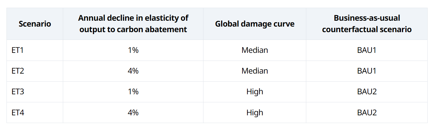
Note: See also Figure 1 for the relationship between scenarios. The annual decline in carbon mitigation costs refers to the annual per cent decline in the elasticity of output to the change in GHG emissions in that scenario relative to the counterfactual one. See section 2.6 for details on the median vs high climate damage curves. For each energy transition scenario, the relevant counterfactual scenario is the one without the energy transition that relies on the same climate damage curve.

38. The other key source of uncertainty concerns the reduction in output associated with mitigating carbon emissions during the transition phase to 2050, with both output and mitigation measured relative to a business-as-usual counterfactual. In the LTM, the output costs of carbon mitigation are given by marginal abatement cost curves (MACCs) that are country specific and based on simulations carried out with ENV-Linkages, a dynamic computable general equilibrium model maintained by the OECD (Château, Dellink and Lanzi, 2014[2]).7 Policy action to mitigate carbon emissions lowers output in the LTM because of the implicit assumption in ENV-Linkages that the counterfactual economy features an efficient allocation of resources, but other outcomes are conceivable (Box 2). Moreover, ENV-Linkages tends to feature higher carbon abatement costs than many other models used to study the energy transition. This is because it does not assume changes in preferences during the transition period (such as for smaller cars/houses or greener diets) that allow for costless adaptation, and because it features some rigidity in capital reallocation, implying costly capital adjustments to carbon mitigation actions during the transition period.

Click to read more